RStan : MCMC サンプラー用ラッパー
Last Change: 12-Dec-2014.
author : qh73xe
これは何?
Rstan とは C++ベースのコンパイラで高速化させたMCMCサンプラーである Stan の R 用 インターフェイスです.BUGS よりもわかりやすい文法で高速な実行ができるようです.
公式サイト: https://github.com/stan-dev/rstan/wiki/RStan-Getting-Started#how-to-install-rstan
導入方法
公式サイトによると以下の R よりコマンドで導入できるそうです.
> source('http://mc-stan.org/rstan/install.R', echo = TRUE, max.deparse.length = 2000)
> install_rstan()
注釈
インストールに失敗する場合
私の環境(OS:OpenSUSE, R: 3.1.2)では上記のコマンドで導入は上手く行きませんでした.
ログを確認すると RcppEigen (Rstan の依存ライブラリでしょう)の導入の際に gcc から以下の警告が出ています.
- -lgfortran が見つかりません
- -lquadmath が見つかりません
まぁ,とりあえず fortran 関係ということはわかりますので必要そうなものを zypper から入れて起きます.
$ sudo zypper install libpng12-devel xorg-x11-libs freeglut-devel gcc gcc-fortran gcc-c++ make
これで上手く導入ができました.
とりあえず使ってみる
何はともあれ無事動くことを確認します. 公式サイトの “Example 1: Eight Schools” を試して見ます.
まず, R の作業ディレクトリに 8schools.stan というファイルを作成します.
data {
  int<lower=0> J; // number of schools
  real y[J]; // estimated treatment effects
  real<lower=0> sigma[J]; // s.e. of effect estimates
}
parameters {
  real mu;
  real<lower=0> tau;
  real eta[J];
}
transformed parameters {
  real theta[J];
  for (j in 1:J)
    theta[j] <- mu + tau * eta[j];
}
model {
  eta ~ normal(0, 1);
  y ~ normal(theta, sigma);
}
続いて R スクリプトを作成します.
上にも書いたように,R の作業ディレクトリの直下に 8schools.stan が必要です.
- BUGS の場合と同じようにモデルは別のスクリプトで記述するようですので
library(rstan)
schools_dat <- list(J = 8,
y = c(28, 8, -3, 7, -1, 1, 18, 12),
sigma = c(15, 10, 16, 11, 9, 11, 10, 18))
fit <- stan(file = '8schools.stan', data = schools_dat,
iter = 1000, chains = 4)
schools_code <- paste(readLines('8schools.stan'), collapse = '\n')
fit1 <- stan(model_code = schools_code, data = schools_dat, iter = 1000, chains = 4)
fit2 <- stan(fit = fit1, data = schools_dat, iter = 10000, chains = 4)
print(fit2)
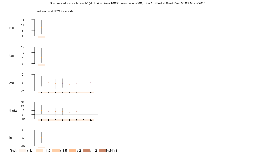
plot(fit2)
結果は以下のようになりました.
Inference for Stan model: schools_code.
4 chains, each with iter=10000; warmup=5000; thin=1;
post-warmup draws per chain=5000, total post-warmup draws=20000.

          mean se_mean   sd   2.5%   25%   50%   75% 97.5% n_eff Rhat
mu        7.90    0.13 5.39  -2.45  4.62  7.89 11.20 18.44  1821    1
tau       6.77    0.14 5.84   0.27  2.54  5.36  9.33 21.97  1837    1
eta[1]    0.40    0.01 0.95  -1.54 -0.23  0.41  1.04  2.24 10770    1
eta[2]    0.00    0.01 0.88  -1.77 -0.57  0.00  0.58  1.74 12111    1
eta[3]   -0.20    0.01 0.92  -1.96 -0.82 -0.22  0.41  1.64  8231    1
eta[4]   -0.04    0.01 0.88  -1.79 -0.62 -0.04  0.55  1.71 12336    1
eta[5]   -0.35    0.01 0.87  -2.06 -0.92 -0.37  0.20  1.40  8771    1
eta[6]   -0.21    0.01 0.89  -1.94 -0.80 -0.22  0.38  1.58 12011    1
eta[7]    0.35    0.01 0.88  -1.41 -0.23  0.37  0.93  2.03 11761    1
eta[8]    0.07    0.01 0.94  -1.78 -0.55  0.07  0.70  1.90 11838    1
theta[1] 11.60    0.13 8.57  -2.19  6.07 10.37 15.70 32.39  4378    1
theta[2]  7.94    0.06 6.42  -4.81  3.97  7.85 11.87 21.15 10047    1
theta[3]  6.05    0.08 7.88 -11.86  1.97  6.60 10.78 19.93  9215    1
theta[4]  7.59    0.06 6.61  -6.08  3.68  7.62 11.66 20.78 12714    1
theta[5]  5.14    0.06 6.41  -9.00  1.33  5.62  9.46 16.36 10345    1
theta[6]  6.07    0.06 6.70  -8.76  2.32  6.50 10.35 18.39 12862    1
theta[7] 10.83    0.10 6.92  -1.20  6.21 10.21 14.76 26.80  5039    1
theta[8]  8.58    0.08 8.01  -7.18  3.92  8.32 12.86 26.48 10360    1
lp__     -4.85    0.04 2.60 -10.57 -6.43 -4.62 -3.00 -0.44  4381    1

Samples were drawn using NUTS(diag_e) at Wed Dec 10 03:46:45 2014.
For each parameter, n_eff is a crude measure of effective sample size,
and Rhat is the potential scale reduction factor on split chains (at conv ergence, Rhat=1).
plot に関しては以下の通りです.